A Brief Introduction to Graphical Models and Bayesian Networks
By Kevin Murphy, 1998.
"Graphical models are a marriage between probability theory and
graph theory. They provide a natural tool for dealing with two problems
that occur throughout applied mathematics and engineering --
uncertainty and complexity -- and in particular they are playing an
increasingly important role in the design and analysis of machine
learning algorithms. Fundamental to the idea of a graphical model is
the notion of modularity -- a complex system is built by combining
simpler parts. Probability theory provides the glue whereby the parts
are combined, ensuring that the system as a whole is consistent, and
providing ways to interface models to data. The graph theoretic side
of graphical models provides both an intuitively appealing interface
by which humans can model highly-interacting sets of variables as well
as a data structure that lends itself naturally to the design of
efficient general-purpose algorithms.
Many of the classical multivariate probabalistic systems studied in
fields such as statistics, systems engineering, information theory,
pattern recognition and statistical mechanics are special cases of the
general graphical model formalism -- examples include mixture models,
factor analysis, hidden Markov models, Kalman filters and Ising
models. The graphical model framework provides a way to view all of
these systems as instances of a common underlying formalism. This view
has many advantages -- in particular, specialized techniques that have
been developed in one field can be transferred between research
communities and exploited more widely. Moreover, the graphical model
formalism provides a natural framework for the design of new systems."
--- Michael Jordan, 1998.
This tutorial
We will briefly discuss the following topics.
- Representation, or, what exactly is a
graphical model?
- Inference, or, how can we use these models
to efficiently answer probabilistic queries?
- Learning, or, what do we do if we don't know what the
model is?
- Decision theory, or, what happens when it
is time to convert beliefs into actions?
- Applications, or, what's this all good for, anyway?
Note: Dan Hammerstrom
has made a pdf version of this web
page.
I also have a closely related tutorial in
postscript or
pdf format.
Articles in the popular press
The following articles provide less technical introductions.
Other sources of technical information
Probabilistic graphical models are graphs in which nodes represent
random variables, and the (lack of) arcs represent conditional
independence assumptions.
Hence they provide a compact representation of joint probability
distributions.
Undirected graphical models, also called Markov
Random Fields (MRFs) or Markov networks,
have a simple definition of independence: two (sets
of) nodes A and B are conditionally independent given a third set, C,
if all paths between the nodes in A and B are separated by a node in C.
By contrast, directed graphical models
also called Bayesian
Networks or Belief Networks (BNs), have a more
complicated notion of independence,
which takes into account the directionality of the
arcs, as we explain below.
Undirected graphical models are more popular with the physics and
vision communities, and directed models are more popular with the AI
and statistics communities. (It is possible to have a model with both
directed and undirected arcs, which is called a chain graph.)
For a careful study of the relationship between directed and
undirected graphical models, see the books by Pearl88, Whittaker90,
and Lauritzen96.
Although directed models have a more complicated notion of
independence than undirected models,
they do have several advantages.
The most important is that
one can regard an arc from A to B as
indicating that A ``causes'' B.
(See the discussion on causality.)
This can be used as a guide to construct the graph structure.
In addition, directed models can encode deterministic
relationships, and are easier to learn (fit to data).
In the rest of this tutorial, we will only discuss directed graphical
models, i.e., Bayesian networks.
In addition to the graph structure, it is necessary to specify the
parameters of the model.
For a directed model, we must specify
the Conditional Probability Distribution (CPD) at each node.
If the variables are discrete, this can be represented as a table
(CPT), which lists the probability that the child node takes on each
of its different values for each combination of values of its
parents. Consider the following example, in which all nodes are binary,
i.e., have two possible values, which we will denote by T (true) and
F (false).
We see that the event "grass is wet" (W=true) has two
possible causes: either the water sprinker is on (S=true) or it is
raining (R=true).
The strength of this relationship is shown in the table.
For example, we see that Pr(W=true | S=true, R=false) = 0.9 (second
row), and
hence, Pr(W=false | S=true, R=false) = 1 - 0.9 = 0.1, since each row
must sum to one.
Since the C node has no parents, its CPT specifies the prior
probability that it is cloudy (in this case, 0.5).
(Think of C as representing the season:
if it is a cloudy season, it is less likely that the sprinkler is on
and more likely that the rain is on.)
The simplest conditional independence relationship encoded in a Bayesian
network can be stated as follows:
a node is independent of its ancestors given its parents, where the
ancestor/parent relationship is with respect to some fixed topological
ordering of the nodes.
By the chain rule of probability,
the joint probability of all the nodes in the graph above is
P(C, S, R, W) = P(C) * P(S|C) * P(R|C,S) * P(W|C,S,R)
By using conditional independence relationships, we can rewrite this as
P(C, S, R, W) = P(C) * P(S|C) * P(R|C) * P(W|S,R)
where we were allowed to simplify the third term because R is
independent of S given its parent C, and the last term because W is
independent of C given its parents S and R.
We can see that the conditional independence relationships
allow us to represent the joint more compactly.
Here the savings are minimal, but in general, if we had n binary
nodes, the full joint would require O(2^n) space to represent, but the
factored form would require O(n 2^k) space to represent, where k is
the maximum fan-in of a node. And fewer parameters makes learning easier.
Are "Bayesian networks" Bayesian?
Despite the name,
Bayesian networks do not necessarily imply a commitment to Bayesian
statistics.
Indeed, it is common to use
frequentists methods to estimate the parameters of the CPDs.
Rather, they are so called because they use
Bayes' rule for
probabilistic inference, as we explain below.
(The term "directed graphical model" is perhaps more appropriate.)
Nevetherless, Bayes nets are a useful representation for hierarchical
Bayesian models, which form the foundation of applied Bayesian
statistics
(see e.g., the BUGS project).
In such a model, the parameters are treated like any other random
variable, and becomes nodes in the graph.
Inference
The most common task we wish to solve using Bayesian networks is
probabilistic inference. For example, consider the water sprinkler
network, and suppose we observe the
fact that the grass is wet. There are two possible causes for this:
either it is raining, or the sprinkler is on. Which is more likely?
We can use Bayes' rule to compute the posterior probability of each
explanation (where 0==false and 1==true).


where

is a normalizing constant, equal to the probability (likelihood) of
the data.
So we see that it is more likely that the grass is wet because
it is raining:
the likelihood ratio is 0.7079/0.4298 = 1.647.
In the above example, notice that the two causes "compete" to "explain" the
observed data. Hence S and R become conditionally dependent given that
their common child, W, is observed, even though they are marginally
independent. For example,
suppose the grass is wet, but that we also know that it is raining.
Then the posterior probability that the sprinkler is on goes down:
Pr(S=1|W=1,R=1) = 0.1945
This is called "explaining away".
In statistics, this is known as Berkson's paradox, or "selection
bias". For a dramatic example of this effect, consider a college which
admits students who are either brainy or sporty (or both!).
Let C denote the event that someone is admitted to college, which is
made true if they are either brainy (B) or sporty (S).
Suppose in the general population, B and S are independent.
We can model our conditional independence assumptions using a graph
which is a V structure, with arrows pointing down:
   B   S
    \ /
     v
     C
Now look at a population of college students (those for which C is
observed to be true).
It will be found that being brainy makes you less likely to be sporty
and vice versa, because either property alone is sufficient to explain
the evidence on C
(i.e., P(S=1 | C=1, B=1) <= P(S=1 | C=1)).
(If you don't believe me,
try this little BNT demo!)
Top-down and bottom-up reasoning
In the water sprinkler example, we had evidence of an effect (wet grass), and
inferred the most likely cause. This is called diagnostic, or "bottom
up", reasoning, since it goes
from effects to causes; it is a common task in expert systems.
Bayes nets can also be used for causal, or "top down",
reasoning. For example, we can compute the probability that the grass
will be wet given that it is cloudy.
Hence Bayes nets are often called "generative" models, because they
specify how causes generate effects.
One of the most exciting things about Bayes nets is that they can be
used to put discussions about causality on a solid mathematical basis.
One very interesting question is: can we distinguish causation from mere
correlation? The answer is "sometimes",
but you need to measure the relationships between at least
three variables; the intution is that one of the variables acts
as a "virtual control" for the relationship between the other two,
so we don't always need to do experiments to infer causality.
See the following books for details.
- "Causality: Models,
Reasoning and Inference",
Judea Pearl, 2000, Cambridge University Press.
- "Causation,
Prediction and Search", Spirtes, Glymour and
Scheines, 2001 (2nd edition), MIT Press.
- "Cause
and Correlation in Biology", Bill Shipley, 2000,
Cambridge University Press.
- "Computation, Causation and Discovery", Glymour and Cooper (eds),
1999, MIT Press.
Conditional independence in Bayes Nets
In general,
the conditional independence relationships encoded by a Bayes Net
are best be explained by means of the "Bayes Ball"
algorithm (due to Ross Shachter), which is as follows:
Two (sets of) nodes A and B are conditionally independent
(d-separated) given a set C
if and only if there is no
way for a ball to get from A to B in the graph, where the allowable
movements of the ball are shown below.
Hidden nodes are nodes whose values
are not known, and are depicted as unshaded; observed nodes (the ones
we condition on) are shaded.
The dotted arcs indicate direction of flow of the ball.
The most interesting case is the first column, when we have two arrows converging on a
node X (so X is a "leaf" with two parents).
If X is hidden, its parents are marginally independent, and hence the
ball does not pass through (the ball being "turned around" is
indicated by the curved arrows); but if X is observed, the parents become
dependent, and the ball does pass through,
because of the explaining away phenomenon.
Notice that, if this graph was undirected, the child
would always separate the parents; hence when converting a directed
graph to an undirected graph, we must add links between "unmarried"
parents who share a common child (i.e., "moralize" the graph) to prevent us reading off incorrect
independence statements.
Now consider the second column in which we have two diverging arrows from X (so X is a
"root").
If X is hidden,
the children are dependent, because they have a hidden common cause,
so the ball passes through.
If X is observed, its children are rendered conditionally
independent, so the ball does not pass through.
Finally, consider the case in which we have one incoming and outgoing
arrow to X. It is intuitive that the nodes upstream
and downstream of X are dependent iff X is hidden, because
conditioning on a node breaks the graph at that point.
Bayes nets with discrete and continuous nodes
The introductory example used nodes with categorical values and multinomial distributions.
It is also possible to create Bayesian networks with continuous valued nodes.
The most common distribution for such variables is the Gaussian.
For discrete nodes with continuous parents, we can use the
logistic/softmax distribution.
Using multinomials, conditional Gaussians, and the softmax
distribution, we can have a rich toolbox for making complex models.
Some examples are shown below. For details, click
here.
(Circles denote continuous-valued random variables,
squares denote discrete rv's, clear
means hidden, and shaded means observed.)
For more details, see this excellent paper.
Dynamic Bayesian Networks (DBNs) are directed graphical models of stochastic
processes.
They generalise hidden Markov models (HMMs)
and linear dynamical systems (LDSs)
by representing the hidden (and observed) state in terms of state
variables, which can have complex interdependencies.
The graphical structure provides an easy way to specify these
conditional independencies, and hence to provide a compact
parameterization of the model.
Note that "temporal Bayesian network" would be a better name than
"dynamic Bayesian network", since
it is assumed that the model structure does not change, but
the term DBN has become entrenched.
We also normally assume that the parameters do not
change, i.e., the model is time-invariant.
However, we can always add extra
hidden nodes to represent the current "regime", thereby creating
mixtures of models to capture periodic non-stationarities.
There are some cases where the size of the state space can change over
time, e.g., tracking a variable, but unknown, number of objects.
In this case, we need to change the model structure over time.
The simplest kind of DBN is a Hidden Markov Model (HMM), which has
one discrete hidden node and one discrete or continuous
observed node per slice. We illustrate this below.
As before, circles denote continuous nodes, squares denote
discrete nodes, clear means hidden, shaded means observed.
We have "unrolled" the model for 4 "time slices" -- the structure and parameters are
assumed to repeat as the model is unrolled further.
Hence to specify a DBN, we need to
define the intra-slice topology (within a slice),
the inter-slice topology (between two slices),
as well as the parameters for the first two slices.
(Such a two-slice temporal Bayes net is often called a 2TBN.)
Some common variants on HMMs are shown below.
A Linear Dynamical System (LDS) has the same topology as an HMM, but
all the nodes are assumed to have linear-Gaussian distributions, i.e.,
   x(t+1) = A*x(t) + w(t),  w ~ N(0, Q),  x(0) ~ N(init_x, init_V)
   y(t)   = C*x(t) + v(t),  v ~ N(0, R)
The Kalman filter is a way of doing online filtering in this model.
Some simple variants of LDSs are shown below.
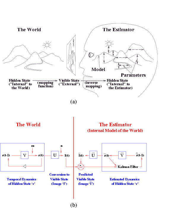
The Kalman filter has been proposed as a model for how the brain
integrates visual cues over time to infer the state of the world,
although the reality is obviously much more complicated.
The main point is not that the Kalman filter is the right model, but that
the brain is combining bottom up and top down cues.
The figure below is from a paper called
"A Kalman Filter Model of the Visual Cortex",
by P. Rao, Neural Computation 9(4):721--763, 1997.
 It is also possible to create temporal models with much more complicated
topologies, such as the Bayesian Automated Taxi (BAT) network shown
below.
(For simplicity, we only show the observed leaves for slice 2.
Thanks to Daphne Koller for providing this figure.)
It is also possible to create temporal models with much more complicated
topologies, such as the Bayesian Automated Taxi (BAT) network shown
below.
(For simplicity, we only show the observed leaves for slice 2.
Thanks to Daphne Koller for providing this figure.)
When some of the observed nodes are thought of as inputs (actions), and some as
outputs (percepts), the DBN becomes a POMDP.
See also the section on decision theory below.
A generative model for generative models
The figure below, produced by Zoubin Ghahramani and Sam Roweis, is a
good summary of the relationships between some popular graphical models.
A graphical model specifies a complete
joint probability distribution (JPD) over all the variables.
Given the JPD, we can answer all possible inference
queries by marginalization (summing out over irrelevant variables), as
illustrated in the introduction. However, the JPD has size O(2^n), where n is the
number of nodes, and we have assumed each node can have 2
states. Hence summing over the JPD takes exponential time.
We now discuss more efficient methods.
For a directed graphical model (Bayes net),
we can sometimes use the factored representation of the JPD
to do marginalisation efficiently.
The key idea is to "push sums in" as far as possible when summing
(marginalizing) out irrelevant terms, e.g., for the water sprinkler network
Notice that, as we perform the innermost sums, we create new terms,
which need to be summed over in turn e.g.,

where

Continuing in this way,

where

This algorithm is called Variable Elimination.
The principle of distributing sums over products can be generalized
greatly to apply to any commutative semiring.
This forms the basis of many common algorithms, such as Viterbi
decoding and the Fast Fourier Transform. For details, see
The amount of work we perform when computing a marginal is bounded by
the size of the largest term that we encounter. Choosing a summation
(elimination) ordering to
minimize this is NP-hard, although greedy algorithms work well in
practice.
Dynamic programming
If we wish to compute several marginals at the same time, we can use Dynamic
Programming (DP) to avoid the redundant computation that would be involved
if we used variable elimination repeatedly.
If the underlying undirected graph of the BN is acyclic (i.e., a tree), we can use a
local message passing algorithm due to Pearl.
This is a generalization of the well-known forwards-backwards
algorithm for HMMs (chains).
For details, see
- "Probabilistic Reasoning in Intelligent Systems", Judea Pearl,
1988, 2nd ed.
- "Fusion and propogation with multiple observations in belief networks",
Peot and Shachter, AI 48 (1991) p. 299-318.
If the BN has undirected cycles (as in the water sprinkler example),
local message passing algorithms run the risk of double counting.
e.g., the information from S and R flowing
into W is not independent, because it came from a common cause, C.
The most common approach is therefore to convert the BN into a tree,
by clustering nodes together, to form what is called a
junction tree, and then running a local message passing algorithm on
this tree. The message passing scheme could be Pearl's algorithm, but
it is more common to use a variant designed for undirected models.
For more details, click here
The running time of the DP algorithms is exponential in the size of
the largest cluster (these clusters correspond to the intermediate
terms created by variable elimination). This size is called the
induced width of the graph. Minimizing this is NP-hard.
Approximation algorithms
Many models of interest,
such as those with repetitive structure, as in
multivariate time-series or image analysis,
have large induced width, which makes exact
inference very slow.
We must therefore resort to approximation techniques.
Unfortunately, approximate inference is #P-hard, but we can nonetheless come up
with approximations which often work well in practice. Below is a list
of the major techniques.
- Variational methods.
The simplest example is the mean-field approximation,
which exploits the law of
large numbers to approximate large sums of random variables by their
means. In particular, we essentially decouple all the nodes, and
introduce a new parameter, called a variational parameter, for each
node, and iteratively update these parameters so as to minimize the
cross-entropy (KL distance) between the approximate and true
probability distributions. Updating the variational parameters becomes a proxy for
inference. The mean-field approximation produces a lower bound on the
likelihood. More sophisticated methods are possible, which give
tighter lower (and upper) bounds.
- Sampling (Monte Carlo) methods. The simplest kind is importance
sampling, where we draw random samples x from P(X), the (unconditional)
distribution on the hidden variables, and
then weight the samples by their likelihood, P(y|x), where y is the
evidence. A more efficient approach in high dimensions is called Monte
Carlo Markov Chain (MCMC), and
includes as special cases Gibbs sampling and the Metropolis-Hasting algorithm.
- "Loopy belief propogation". This entails
applying Pearl's algorithm to the original
graph, even if it has loops (undirected cycles).
In theory, this runs the risk of double counting, but Yair Weiss and
others have proved that in certain cases (e.g., a single loop), events are double counted
"equally", and hence "cancel" to give the right answer.
Belief propagation is equivalent to exact inference on a modified
graph, called the universal cover or unwrapped/ computation tree,
which has the same local topology as the original graph.
This is the same as the Bethe and cavity/TAP approaches in statistical
physics.
Hence there is a deep connection between
belief propagation and variational methods that people are currently investigating.
- Bounded cutset conditioning. By instantiating subsets of the variables,
we can break loops in the graph.
Unfortunately, when the cutset is large, this is very slow.
By instantiating only a subset of values of the cutset, we can compute
lower bounds on the probabilities of interest.
Alternatively, we can sample the cutsets jointly, a technique known as block Gibbs sampling.
- Parametric approximation methods.
These express the intermediate summands in a simpler
form, e.g., by approximating them as a product of smaller factors.
"Minibuckets" and the Boyen-Koller algorithm fall into this category.
Approximate inference is a huge topic:
see the references for more details.
Inference in DBNs
The general inference problem for DBNs is to compute
P(X(i,t0) | y(:, t1:t2)), where X(i,t) represents the i'th hidden
variable at time and t Y(:,t1:t2) represents all the evidence
between times t1 and t2.
(In fact, we often also want to compute joint distributions of
variables over one or more time slcies.)
There are several special cases of interest, illustrated below.
The arrow indicates t0: it is X(t0) that we are trying to estimate.
The shaded region denotes t1:t2, the available data.
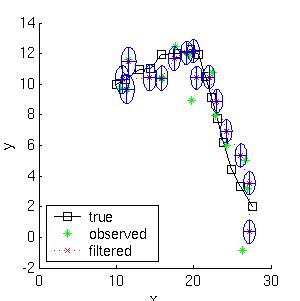
Here is a simple example of inference in an LDS.
Consider a particle moving in the plane at
constant velocity subject to random perturbations in its trajectory.
The new position (x1, x2) is the old position plus the velocity (dx1,
dx2) plus noise w.
[ x1(t)  ] =  [1 0 1 0] [ x1(t-1)  ] + [ wx1  ]
[ x2(t)  ]    [0 1 0 1] [ x2(t-1)  ]   [ wx2  ]
[ dx1(t) ]    [0 0 1 0] [ dx1(t-1) ]   [ wdx1 ]
[ dx2(t) ]    [0 0 0 1] [ dx2(t-1) ]   [ wdx2 ]
We assume we only observe the position of the particle.
[ y1(t) ] =  [1 0 0 0] [ x1(t)  ] + [ vx1 ]
[ y2(t) ]    [0 1 0 0] [ x2(t)  ]   [ vx2 ]
                       [ dx1(t) ]
                       [ dx2(t) ]
Suppose we start out at position (10,10) moving to the right with
velocity (1,0).
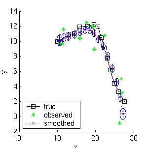
We sampled a random trajectory of length 15.
Below we show the filtered and smoothed trajectories.
The mean squared error of the filtered estimate is 4.9; for the
smoothed estimate it is 3.2.
Not only is the smoothed estimate better, but we know that
it is better, as illustrated by the smaller uncertainty ellipses;
this can help in e.g., data association problems.
Note how the smoothed ellipses are larger at the ends, because these
points have seen less data. Also, note how rapidly the filtered
ellipses reach their steady-state (Ricatti) values.
(See my Kalman
filter toolbox for more details.)
One needs to specify two things to describe a BN: the graph topology
(structure) and the parameters of each CPD. It is possible to learn
both of these from data. However, learning structure is much harder
than learning parameters. Also, learning when some of the nodes are
hidden, or we have missing data, is much harder than when everything
is observed. This gives rise to 4 cases:
Structure   Observability    Method
---------------------------------------------
Known       Full             Maximum Likelihood Estimation
Known       Partial          EM (or gradient ascent)
Unknown     Full             Search through model space
Unknown     Partial          EM + search through model space
We assume that the goal of learning in this case is to find the values
of the parameters of each CPD which maximizes the likelihood of the
training data,
which contains N cases (assumed to be independent).
The normalized log-likelihood of the training set D
is a sum of terms, one
for each node:
 We see that the log-likelihood scoring function decomposes
according to the structure of the graph, and hence we can maximize the
contribution to the log-likelihood of each node independently
(assuming the parameters in each node are independent of the other nodes).
We see that the log-likelihood scoring function decomposes
according to the structure of the graph, and hence we can maximize the
contribution to the log-likelihood of each node independently
(assuming the parameters in each node are independent of the other nodes).
Consider estimating the Conditional Probability Table for the W
node. If we have a set of training data, we can just count the number
of times the grass is wet when it is raining and the sprinler is on,
N(W=1,S=1,R=1), the number of times the grass is wet when it is
raining and the sprinkler is off, N(W=1,S=0,R=1), etc. Given these
counts (which are the sufficient statistics), we can find the Maximum
Likelihood Estimate of the CPT as follows:

where the denominator is N(S=s,R=r) = N(W=0,S=s,R=r) + N(W=1,S=s,R=r).
Thus "learning" just amounts to counting (in the case of multinomial
distributions).
For Gaussian nodes, we can compute the sample mean and variance, and
use linear regression to estimate the weight matrix.
For other kinds of distributions, more complex procedures are
necessary.
As is well known from the HMM literature, ML estimates of CPTs are
prone to sparse data problems, which can be solved by using (mixtures
of) Dirichlet priors (pseudo counts).
This results in a Maximum A Posteriori (MAP) estimate.
For Gaussians, we can use a Wishart prior, etc.
When some of the nodes are hidden, we can use the EM (Expectation
Maximization) algorithm to find a (locally) optimal Maximum Likelihood
Estimate of the parameters.
The basic idea behind EM is that, if we knew the values of
all the nodes, learning (the M step) would be easy, as we saw
above. So in the E step, we compute the expected values of all the
nodes using an inference algorithm, and then treat these expected
values as though they were observed (distributions). For example, in the case
of the W node, we replace the observed counts of the events with the number of times
we expect to see each event:
P(W=w|S=s,R=r) = E N(W=w,S=s,R=r) / E N(S=s,R=r)
where
E N(x) is the expected number of times event x
occurs in the whole training set, given the current guess of the parameters.
These expected counts can be computed as follows
E N(.) = E sum_k I(. | D(k)) = sum_k P(. | D(k))
where I(x | D(k)) is an indicator function which is 1 if event
x occurs in training case k, and 0 otherwise.
Given the expected counts, we maximize the parameters, and then
recompute the expected counts, etc. This iterative procedure is
guaranteed to converge to a local maximum of the likelihood surface.
It is also possible to do gradient ascent on the likelihood surface (the
gradient expression also involves the expected counts), but EM is
usually faster (since it uses the natural gradient) and simpler (since
it has no step size parameter and
takes care of parameter constraints (e.g., the "rows" of the
CPT having to sum to one) automatically).
In any case, we see than when nodes are hidden, inference becomes a
subroutine which is called by the learning procedure; hence fast
inference algorithms are crucial.
We start by discussing the scoring function which we use to select
models; we then discuss algorithms which attempt to optimize this
function over the space of models, and finally examine their computational and
sample complexity.
The maximum likelihood model will be a
complete graph, since this has the largest
number of parameters, and hence can fit the data the best.
A well-principled way to avoid this kind of over-fitting is to put a prior on models,
specifying that we prefer sparse models.
Then, by Bayes' rule, the MAP model is the one that maximizes
 Taking logs, we find
 where c = - \log \Pr(D) is a constant independent of G.
The effect of the structure prior P(G) is equivalent to penalizing overly complex
models.
However, this is not strictly necessary, since the marginal likelihood
term
P(D|G) = \int_{\theta} P(D|G, \theta)
has a similar effect of penalizing models with too many parameters
(this is known as Occam's razor).
The goal of structure learning is to learn a dag (directed acyclic
graph) that best explains the data. This is an NP-hard problem, since
the number of dag's on N variables is super-exponential in N. (There is no closed
form formula for this, but to give you an idea,
there are 543 dags on 4 nodes, and O(10^18) dags on 10 nodes.)
If we know the ordering of the nodes, life becomes much simpler,
since we can learn the parent set for
each node independently
(since the score is decomposable), and we don't need to worry about acyclicity constraints.
For each node, there at most
\sum_{k=0}^n \choice{n}{k} = 2^n
sets of possible parents for each node, which can be
arranged in a lattice as shown below for n=4.
The problem is to find the highest scoring point in this lattice.
There are three obvious ways to search this graph: bottom up, top
down, or middle out.
In the bottom up approach, we
start at the bottom of the
lattice, and evaluate the score at all points in each successive
level.
We must decide whether the gains in score produced by a
larger parent set is ``worth it''.
The standard approach in the reconstructibility analysis (RA) community uses the fact
that \chi^2(X,Y) \approx I(X,Y) N \ln(4), where N is the number of
samples and I(X,Y) is the mutual information (MI) between X and Y.
Hence we can use a \chi^2 test to decide
whether an increase in the MI score is statistically significant.
(This also gives us some kind of confidence measure on the connections
that we learn.)
Alternatively, we can use a BIC score.
Of course, if we do not know if we have achieved the maximum possible
score, we do not know when to stop searching, and hence we must
evaluate all points in the lattice (although we can obviously use
branch-and-bound). For large n, this is
computationally infeasible, so a common approach is to only search up
until level K (i.e., assume a bound on the maximum number of parents
of each node), which takes O(n ^ K) time.
The obvious way to avoid the exponential cost (and the need for a
bound, K) is to use heuristics to
avoid examining all possible subsets.
(In fact, we must use heuristics of some kind, since the problem of
learning optimal structure is NP-hard \cite{Chickering95}.)
One approach in the RA framework, called Extended Dependency Analysis (EDA)
\cite{Conant88}, is as follows.
Start by evaluating all subsets of size up to two, keep all the ones with
significant (in the \chi^2 sense) MI with the target node, and take the union of the resulting set
as the set of parents.
The disadvantage of this greedy technique is that it will fail to find a set
of parents unless some subset of size two has significant MI with the
target variable. However, a Monte Carlo
simulation in \cite{Conant88} shows that most random relations have
this property.
In addition, highly interdependent sets of parents (which might
fail the pairwise MI test) violate the causal
independence assumption, which is necessary to justify the use of
noisy-OR and similar CPDs.
An alternative technique, popular in the UAI community, is to start
with an initial guess of the model structure (i.e., at a specific
point in the lattice), and then perform local
search, i.e., evaluate the score of neighboring points in the lattice,
and move to the best such point, until we reach a local optimum. We
can use multiple restarts to try to find the global optimum, and to
learn an ensemble of models.
Note that, in the partially observable case, we need to have an
initial guess of the model structure in order to estimate the values
of the hidden nodes, and hence the (expected) score of each model; starting with the fully
disconnected model (i.e., at the bottom of the lattice) would be a bad
idea, since it would lead to a poor estimate.
Finally, we come to the hardest case of all, where the structure is
unknown and there are hidden variables and/or missing data.
In this case, to compute the Bayesian score, we must marginalize out
the hidden nodes as well as the parameters.
Since this is usually intractable, it is common to usean asymptotic
approximation to the posterior called BIC (Bayesian Information
Criterion), which is defined as follows:
\log \Pr(D|G) \approx \log \Pr(D|G, \hat{\Theta}_G) - \frac{\log N}{2} \#G
where N is the number of samples,
\hat{\Theta}_G is the ML estimate of the parameters,
and
#G is the dimension of the model.
(In the fully observable case, the dimension of a model is the number
of free parameters. In a model with hidden variables, it might be less
than this.)
The first term is just the likelihood and
the second term is a penalty for model complexity.
(The BIC score is identical to the Minimum Description Length (MDL)
score.)
Although the BIC score decomposes into a sum of local terms, one per
node,
local search is still expensive, because we need to run EM at each
step to compute \hat{\Theta}. An alternative approach is to do the
local search steps inside of the M step of EM - this is called
Structureal EM, and provably converges to a local maximum of the BIC
score (Friedman, 1997).
So far, structure learning has meant finding the right connectivity
between pre-existing nodes. A more interesting problem is inventing
hidden nodes on demand. Hidden nodes can make a model much more
compact, as we see below.
 (a) A BN with a hidden variable H. (b) The simplest network
that can capture the same distribution without using a hidden variable
(created using arc reversal and node elimination).
If H is binary and the other nodes are trinary, and we assume full
CPTs, the first network has 45 independent parameters, and the second
has 708.
(a) A BN with a hidden variable H. (b) The simplest network
that can capture the same distribution without using a hidden variable
(created using arc reversal and node elimination).
If H is binary and the other nodes are trinary, and we assume full
CPTs, the first network has 45 independent parameters, and the second
has 708.
The standard approach is to keep adding
hidden nodes one at a time, to some part of the network (see below),
performing structure learning at each
step, until the score drops.
One problem is choosing the cardinality (number of possible values)
for the hidden node, and its type of CPD.
Another problem is
choosing where to add the new hidden node.
There is no point making it a child, since hidden children can always
be marginalized away, so we need to find an existing node which needs
a new parent, when the current set of possible parents is not adequate.
\cite{Ramachandran98} use the following heuristic for finding nodes
which need new parents: they consider
a noisy-OR node which is nearly always on, even if its non-leak
parents are off, as an
indicator that there is a missing parent.
Generalizing this technique beyond noisy-ORs is an interesting open
problem.
One approach might be to examine
H(X|Pa(X)):
if this is very high, it means the current set of parents are
inadequate to ``explain'' the residual entropy; if Pa(X) is the
best (in the BIC or \chi^2 sense) set of parents we have been able
to find in the current model, it
suggests we need to create a new node and add it to Pa(X).
A simple heuristic for inventing hidden nodes in the case of DBNs is
to check if the Markov property is being violated for any particular
node. If so, it suggests that we need connections to slices further
back in time. Equivalently, we can add new lag variables
and connect to them.
Of course,
interpreting the ``meaning'' of hidden nodes is always
tricky, especially since they are often unidentifiable,
e.g., we can often switch the interpretation of the true and false states
(assuming for simplicity that the hidden node is binary) provided we
also permute the parameters appropriately. (Symmetries such as this are
one cause of the multiple maxima in the likelihood surface.)
The following are good tutorial articles.
It is often said that "Decision Theory = Probability Theory + Utility
Theory".
We have outlined above how we can model joint probability distributions in a
compact way by using sparse graphs to reflect conditional independence
relationships.
It is also possible to decompose multi-attribute utility functions in
a similar way:
we create a node for each term in the sum, which
has as parents all the attributes (random
variables) on which it depends; typically, the utility node(s) will
have action node(s) as parents, since the utility depends both on the
state of the world and the action we perform.
The resulting graph is called an influence diagram.
In principle, we can then use the influence diagram to compute
the optimal (sequence of) action(s) to perform so as to maximimize
expected utility, although this is computationally intractible for all
but the smallest problems.
Classical control theory is mostly concerned with the special case
where the graphical model is a
Linear Dynamical System
and the utility function is negative quadratic loss, e.g., consider a
missile tracking an airplane: its goal is to minimize the squared
distance between itself and the target. When the utility function
and/or the system model becomes more complicated, traditional methods
break down, and one has to use reinforcement learning to find the
optimal policy (mapping from states to actions).
The most widely used Bayes Nets are undoubtedly the ones embedded in
Microsoft's products, including the Answer
Wizard of Office 95, the Office Assistant (the bouncy paperclip guy) of
Office 97, and over 30 Technical Support Troubleshooters.
BNs originally arose out of an attempt to add probabilities to
expert systems, and this is still the most common use for BNs.
A famous example is
QMR-DT, a decision-theoretic reformulation of the Quick Medical
Reference (QMR) model.
 Here, the top layer represents hidden disease nodes, and the bottom
layer represents observed symptom nodes.
The goal is to infer the posterior probability of each disease given
all the symptoms (which can be present, absent or unknown).
QMR-DT is so densely connected that exact inference is impossible. Various approximation
methods have been used, including sampling, variational and loopy
belief propagation.
Here, the top layer represents hidden disease nodes, and the bottom
layer represents observed symptom nodes.
The goal is to infer the posterior probability of each disease given
all the symptoms (which can be present, absent or unknown).
QMR-DT is so densely connected that exact inference is impossible. Various approximation
methods have been used, including sampling, variational and loopy
belief propagation.
Another interesting fielded application is the
Vista system, developed
by Eric Horvitz.
The Vista system is a decision-theoretic system that has been used at
NASA Mission Control Center in Houston for several years. The system
uses Bayesian networks to interpret live telemetry and provides advice
on the likelihood of alternative failures of the space shuttle's
propulsion systems. It also considers time criticality and recommends
actions of the highest expected utility. The Vista system also employs
decision-theoretic methods for controlling the display of information
to dynamically identify the most important information to highlight.
Horvitz has gone on to attempt to apply similar technology to
Microsoft products, e.g., the Lumiere project.
Special cases of BNs were independently invented by many different
communities, for use in e.g., genetics (linkage analysis), speech
recognition (HMMs), tracking (Kalman fitering), data compression
(density estimation)
and coding (turbocodes), etc.
For examples of other applications, see the
special issue of Proc. ACM 38(3), 1995,
and the Microsoft
Decision Theory Group page.
Applications to biology
This is one of the hottest areas.
For a review, see
In reverse chronological order (bold means particularly recommended)
- F. V. Jensen.
"Bayesian Networks and Decision Graphs".
Springer.
2001.
Probably the best introductory book available.
-
D. Edwards.
"Introduction to Graphical Modelling", 2nd ed.
Springer-Verlag.
2000.
Good treatment of undirected graphical models from a statistical perspective.
- J. Pearl.
"Causality".
Cambridge.
2000.
The definitive book on using causal DAG modeling.
- R. G. Cowell, A. P. Dawid, S. L. Lauritzen and
D. J. Spiegelhalter.
"Probabilistic Networks and Expert Systems".
Springer-Verlag.
1999.
Probably the best book available,
although the treatment is restricted to
exact inference.
- M. I. Jordan (ed).
"Learning in Graphical Models".
MIT Press.
1998.
Loose collection of papers on machine learning, many related to
graphical models.
One of the few books to discuss approximate inference.
- B. Frey.
"Graphical models for machine learning and digital communication",
MIT Press.
1998.
Discusses pattern recognition and turbocodes using (directed)
graphical models.
- E. Castillo and J. M. Gutierrez and A. S. Hadi.
"Expert systems and probabilistic network models".
Springer-Verlag, 1997.
A Spanish
version is available online for free.
- F. Jensen.
"An introduction to Bayesian Networks".
UCL Press.
1996.
Out of print.
Superceded by his 2001 book.
- S. Lauritzen.
"Graphical Models",
Oxford.
1996.
The definitive mathematical exposition of the theory of graphical
models.
- S. Russell and P. Norvig.
"Artificial Intelligence: A Modern Approach".
Prentice Hall.
1995.
Popular undergraduate textbook that includes a readable chapter on
directed graphical models.
- J. Whittaker.
"Graphical Models in Applied Multivariate Statistics",
Wiley.
1990.
This is the first book published on graphical modelling from a statistics
perspective.
- R. Neapoliton.
"Probabilistic Reasoning in Expert Systems".
John Wiley & Sons.
1990.
- J. Pearl.
"Probabilistic Reasoning in Intelligent Systems: Networks of Plausible Inference."
Morgan Kaufmann.
1988.
The book that got it all started!
A very insightful book, still relevant today.
Review articles
Exact Inference
- C. Huang and A. Darwiche, 1996.
"Inference in Belief Networks: A procedural guide",
Intl. J. Approximate Reasoning, 15(3):225-263.
- R. McEliece and S. M. Aji, 2000.
The Generalized Distributive Law,
IEEE Trans. Inform. Theory, vol. 46, no. 2 (March 2000),
pp. 325--343.
- F. Kschischang, B. Frey and H. Loeliger, 2001.
Factor
graphs and the sum product algorithm,
IEEE Transactions on Information Theory, February, 2001.
- M. Peot and R. Shachter, 1991.
"Fusion and propogation with multiple observations in belief networks",
Artificial Intelligence, 48:299-318.
Approximate Inference
Learning
DBNs