


Real evolution finds the right direction by trying and eliminating many wrong ones. It is not known to have a memory of the previous changes that were successful. Instead, many individuals are generated that have particular characteristics in different dimensions. The individuals that have moved in the wrong direction are simply eliminated. There is an excessive number of individuals at nature's disposal, and there is nothing wrong with wasting a few. However, for an optimization algorithm of practical value, every time step is valuable. Instead of wasting resources by using a large population, I propose gaining efficiency with a short term memory.
Note that in Figure  , the right direction to move could be
discovered by summing a few successful steps. This is exactly the approach
that will be taken.
, the right direction to move could be
discovered by summing a few successful steps. This is exactly the approach
that will be taken.
Adding up too many vectors, however, is dangerous. In Figure ,
things would have worked fine, because there is one right direction to go, but
for a function like Rosenbrock's saddle in Figure , the right
direction is constantly changing. Experiments with high dimensional
optimization problems suggest that, the turning ridge problem is a common one.
Thus, the algorithm should be able to adapt itself to the local terrain it is
moving through.
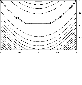
Figure:
Rosenbrock's saddle. The function has a ridge along y = x^2 that rises
slowly as it is traversed from (-1, 1) to (1, 1). The arrows show the steps
taken by the improved Local-Optimize
. Note how the steps shrink in
order to discover a new direction, and grow to speed up once the direction is
established.
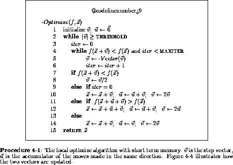
Figure:
An illustration of how Procedure 4-1 uses the vectors u and v.
In (A) the step vector v keeps growing in the same direction as long as
better points are found. u accumulates the moves made in this
direction. Once v fails, the algorithm tries new directions. In (B) a
new direction has been found. The combination u+v is tried and
found to give a better point. In this case u starts accumulating moves
in this new direction. In (C) u+v did not give a better point.
Thus we start moving in the last direction we know that worked, in this case
v.
The Local-Optimize
in Procedure 3-1 of the previous section, is able to
adapt its step sizes to the local terrain. Procedure 4-1 gives an improved
version which is able to adapt its direction also. The local optimizer moves
along its best estimate of the gradient direction. Vector u is used to
accumulate moves made along this direction. When this direction fails, vector
v enters its random probing mode, and searches until it can find a new
direction that works. When a new direction is found, the algorithm tries
u+v as a new estimate of the gradient direction. Either this
succeeds, and u starts accumulating moves along u+v, or
it fails and the new v becomes the new estimate. Figure
explains the algorithm in pictures. As shown in the figure, the algorithm
keeps adapting its estimate of the gradient vector according to the local
terrain.
The performance of the algorithm improved by
an order of magnitude better in complex spaces. Figure is
the result of running this algorithm on Rosenbrock's saddle. The function
has a ridge along the y=x^2 parabola that gradually rises from (-1,1)
to (1,1). The global maximum is at (1,1) and the algorithm was started on
the other end of the ridge, so that it had to traverse the whole parabola.
As illustrated in Figure the more adaptive Procedure 4-1 is
more than an order of magnitude efficient than Procedure 3-1 of the last
chapter.
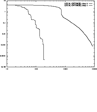
Figure:
Comparison of the two versions of Local-Optimize
from chapter 3 and
chapter 4 on Rosenbrock's saddle. Note that both axes are logarithmic. The
old version converges in 8782 iterations, the new version finds a better value
in 197 iterations.