In this section we describe four experiments of increasing complexity.
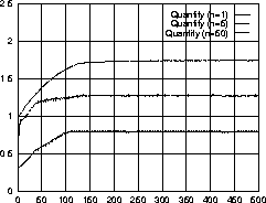
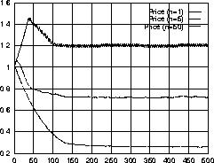
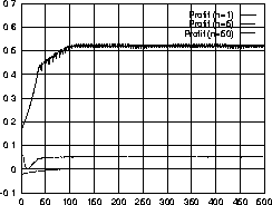
Figure 1 shows how the market reacts to an increase in the size of the private sector. We present plots of total quantity produced in the market, average price and average profit under a monopoly (n=1), an oligopoly (n=5) and perfect competition (n=50). We observe that quantity increases as price and profits fall when the number of firms in the market increases. This is exactly what is predicted by economic theory: competition increases the quantity produced and decreases the average profits in the industry.


This set of simulations shows a state owned enterprise (SOE)
coexisting with a fixed number of identical firms. We observe how the
behavior of the SOE, which has to maintain employment in the industry
above ![]() ,
changes when the number of private firms in the
industry changes.
,
changes when the number of private firms in the
industry changes.
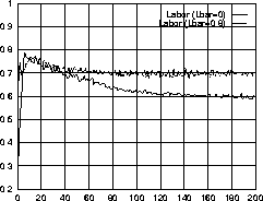
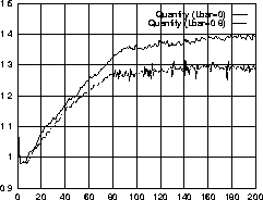
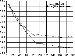
Figure 2 shows how the SOE's employment constraint affects
the total labor employed by the industry, total quantity and average
price. Without a labor constraint, the equilibrium labor usage is
approximately 0.6. When ![]() is set to 0.8, the SOE is forced to
employ more labor than it would have liked and total labor usage in
the industry increases but remains below 0.8 due to averaging errors
in the calculation. The labor constraint is binding which results in a
less efficient outcome, illustrated by a lower equilibrium quantity
and a higher equilibrium price.
is set to 0.8, the SOE is forced to
employ more labor than it would have liked and total labor usage in
the industry increases but remains below 0.8 due to averaging errors
in the calculation. The labor constraint is binding which results in a
less efficient outcome, illustrated by a lower equilibrium quantity
and a higher equilibrium price.
This set of experiments differs from the first experiment in one important sense: firms are allowed to enter and exit the market.
Figure 3 shows how our simulated economy smoothly transitions from a protected environment to perfect competition. During the first 500 periods, entry into this market is prohibited and the SOE is the only firm in the industry (i.e., n=1). The market is liberalized in the 501st period. High profits attract new firms and we observe an increase in the number of firms. This reduces firms' profits. In addition, quantity increases as the price declines. These findings are consistent with economic theory. All of the firms are identical to the SOE in this experiment and a minimum employment constraint is not imposed. The SOE's production can be approximated by dividing total quantity by the number of firms in the industry. The SOE's price and profit are almost identical to the average price and average profit in Figure 3. The significance of this experiment is that the simple SOE agent exhibits monopoly and competitive behavior in an emergent and endogenous manner. The SOE's behavior rules are the same in both monopoly and competitive environments. It is the interaction with the other agents that causes the decline in average price.
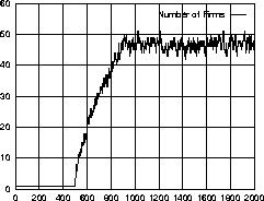
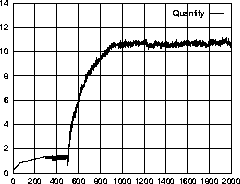
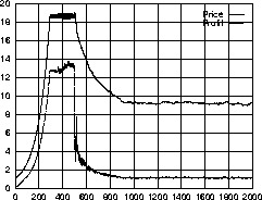
The SOE operates alone for the first 500 periods and reaches the monopoly equilibrium. These 500 periods simulate the centrally planned interval of a transition economy. After 500 periods, the market is liberalized and other firms start entering because of high profits in the industry. The probability that a new firm will want to join the market during a period is an increasing function of average profits in the market. Firms only produce in the feasible region of their supply function, so they never make negative profits. If they do not produce for two periods in a row, they exit the market. For these experiments, the SOE does not have an employment constraint because we discovered that, in the scenarios we analyzed, it was rarely binding.
In Figure 4, the heterogeneity of the firms enables us to observe how price and wage evolve as the industry becomes increasingly dominated by more efficient firms. Rent and wage follow a similar pattern so we only provide a plot for wage. Initial entrants to the market are not necessarily very efficient, because with a high profit margin even inefficient firms can survive. Competition results in lower prices, reducing profit margins so only those firms with more efficient production technologies enter the market as price declines and the inefficient firms exit. As more efficient firms enter the market, labor and capital become more productive so wage and rent are bid up.
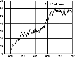
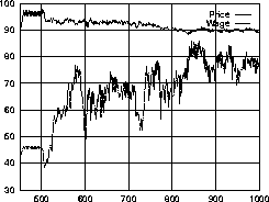
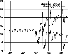
Figure 5 shows the U-shaped output curve that immediately follows liberalization. The U-shaped pattern of output was observed in the transition economies in Eastern Europe and still puzzles economists. The simulation allows us to vary a large number of parameters, and we are able to replicate this result qualitatively for certain ranges of parameter values.
The decline in output after liberalization is due to a decline in the output of the SOE which is not offset by the output of new private firms. The initial entrants to the market are inefficient, and they lure resources away from the more efficient SOE. This is the reason for the initial decline in quantity, the corresponding fall in wage, and rent (not shown here).
Econometric evidence suggests that the start of growth is due to improved resource allocation, both within SOEs and through utilization of assets by new private firms as SOEs are downsized or liquidated [Barbone, Marchetti, & Paternostro1996,Pinto, Belka, & Krajewski1993].
This is illustrated here as well. The increase in quantity coincides with the increase in the efficiency of new firms. At the end of each period, one firm can enter but more than one firm can exit. As a result, n initially increases steadily because even inefficient firms can enter and survive. Later on, n declines as firms exit in large numbers and entry to the market becomes less frequent. As more efficient firms dominate the market, inefficient firms exit and the average price declines. In Figure 4, the equilibrium has not been reached yet, but the declining trend in average price is apparent. The increases in rent and quantity show that the greater efficiency in production increases the total quantity produced and the prices of the inputs.
