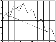
Figure: Starting with large steps is helpful for ignoring small local maxima at the initial stage of the search.


Changing the step size according to recent performance adapts the scale of the search to the local terrain in the search space. It does not only move from coarse grained search to fine grained search, but it is able to re-expand if the function becomes flatter. There are many situations in which, adapting step sizes helps the algorithm be more efficient and robust. First, by starting with large step sizes, the algorithm is able to ignore the small local maxima at the initial stage of the search. Secondly, in simple functions, changing the step size in multiples of 2, leads to logarithmic behavior in the distance to the maximum. This is standard in typical line-search techniques, however my algorithm does not restrict itself to a line and adapts its direction -- as will be explained in the next chapter -- simultaneously with the step size. By not diving into detailed line minimizations, the algorithm is able to locate promising regions faster. Finally, a smaller step size may help determine the right direction. Once a good direction is found, the algorithm can move faster by expanding again.

Figure:
Starting with large steps is helpful for ignoring small local maxima at the
initial stage of the search.
Figure  illustrates the advantage of adapting step sizes in the
presence of many local maxima. Taking different sized steps from A, the
algorithm can discover that the function is decreasing in the immediate
neighborhood (1), it is increasing in the medium scale (2), or that the general
direction is down (3). Starting with a coarse scale lets the algorithm ignore
the low level detail of the search space and discover general regions that are
promising. By ignoring the small peaks, the algorithm in effect performs
gradient ascent on a much smoothed function. As the scale becomes finer
grained, small step sizes give the exact location of the peaks.
The number of steps it takes a hill climber to traverse a path, is linear in
the length of the path, if it is using constant step sizes. In contrast,
Local-Optimize
, by changing the size of its steps in multiples of 2,
requires logarithmic time. For problems where the solution consists of
traveling a certain distance in each dimension, this gives us a simple running
time of:
O(#dimensions x log2(distance))
However, this is not the main advantage. There are several algorithms in the literature [Dennis and Schnabel, 1983,Polak, 1971] that do better under certain assumptions about their objective function. Typical numerical optimization algorithms perform a sequence of line optimizations when faced with high dimensional problems. The advantage of this algorithm is the fact that it does not perform line optimizations. The best value of a certain parameter might change with the settings of the other parameters. In the genetic algorithms literature, this situation is referred to as ``epistasis'', which means the suppression of the effect of a gene by a nonallelic gene. Mathematically, epistasis corresponds to the class of fitness functions that are not additively separable. Such functions are common in optimization problems. Thus, an early convergence of the optimization in order to find the exact maximum on a line may prove useless. Performing a full line-search contradicts with the idea of moving from coarse grained search to fine grained search, and starts fine tuning before the rough picture is ready.


