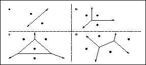
Figure: Voronoi diagrams: Each region consists of points that are closest to the point inside that region.


In the previous section I basically stated the objective of the procedure Distant-Point . More precisely, given a number of points in a bounded space, Distant-Point should find a new point that has the maximum distance to its nearest neighbor. The known algorithms tend to explode in high dimensional spaces. One of the motives behind the method proposed in this thesis is being scalable to problems with high number of dimensions. Thus a simple algorithm which has linear cost is proposed. Another approach is to choose a few random points and pick the best one in diversity as the new starting point. It is shown that in very high number of dimensions, the distance of a random point to its nearest neighbor is very likely to be close to the maximum.

Figure:
Voronoi diagrams: Each region consists of points that are closest to the
point inside that region.
The problem is related to the nearest neighbor problem [Teng, 1994]. Thus it
is no surprise that Voronoi diagrams which are generally used in finding
nearest neighbors are also the key in solving the distant point problem.
Figure  illustrates the basic principle in two dimensions.

Figure:
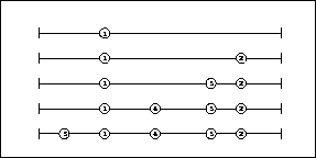
Execution of the distant point algorithm in one dimension. First the largest
interval between the existing points is found, then a random point within that
interval is returned.
A Voronoi diagram consists of convex regions that enclose every given point. Each convex region is the set of points that are closest to the given point in that region. Thus the distant point has to lie on one of the borders. More specifically it will be on one of the corners of the convex Voronoi regions. So a procedure that gives provably correct results, is to check all corners exhaustively, and report the one that maximizes distance to its nearest neighbor. However the number of corners in a Voronoi diagram increase very rapidly with the number of dimensions. Thus this procedure is impractical if the number of dimensions exceed a few.
To cope with high dimensional spaces a more efficient approximation algorithm
is necessary. Figure  demonstrates a solution in one dimension.
Each time a new point is required, the algorithm finds the largest interval
between the existing points. It then returns a random point within that
interval. A simple extension of this to high number of dimensions is to repeat
the same process independently for each dimension and construct the new point
from the values obtained. Although this scheme does not give the optimum
answer, it is observed to produce solutions that are sufficiently distant from
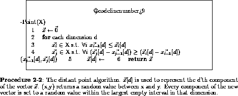
remembered local maxima. Procedure 2-2 is the pseudo-code for this algorithm.


Figure:
The comparison of spheres and half spheres in different number of dimensions
Another option is to choose the new points randomly. Analysis shows that in a
very high dimensional space, the distance of a randomly selected point to its
nearest neighbor will be close to maximum with very high probability. To
simplify the argument, let us assume that the search space has the shape of a
sphere, and that we have found one local maximum at the center. The question
is, how far away a chosen random point will fall. Figure  compares
the radii of spheres in different number of dimensions with their half sized
spheres. Note how the border of the half sized sphere approaches the large one
as the number of dimensions grow. The probability of a random point falling
into a certain region is proportional to the volume of that region. For
example, if a random point is chosen in a ten dimensional space, there is a 0.5
probability of it falling into the narrow strip between the two spheres. Thus,
with high probability, it will be away from the center, and close to the
border. We can extend this argument to spaces of different shapes with more
local maxima in them. The important conclusion is that, if a problem has many
dimensions, it is not worthwhile to spend much effort to find the optimal
distant point. A point randomly chosen is likely to be sufficiently distant.
In the results I present in this thesis, I preferred to use the Distant-Point algorithm presented in Procedure 2-2 for low dimensional problems. For problems with a high number of dimensions (e.g. the molecule energy minimization problem with 153 dimensions), I chose random points instead.


