


There is recent study in mathematical geophysics, on assessing the structure of sedimentary deposits using refraction seismic data [Williamson, 1990]. The synthetic example we have worked on is a rectangular section of earth that is 8000 meters long and 500 meters deep. There are 15 sources and 41 receivers for a total of 615 seismic rays. The path a ray follows depends on the seismic velocity structure in the 2-D section. The domain is divided into a rectangular grid and a seismic velocity value is defined at each node of this grid. In our example we used a grid of 9 by 5 nodes. The 45 seismic velocity values are the parameters of the objective function. The objective function is a ray-tracing algorithm. The algorithm simulates the propagation of the seismic rays from the sources to the receivers. The squared difference in time between the travel times of the simulated rays and a real data set is the output of the objective function.
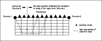
Figure:
The problem of non-separability in refraction tomography. The variation in
just the value at node A effects a part of the domain for one source and the
remaining part for the other.
This problem is a nice example of non-separability. A change in just
one of the parameters will affect all of the domain on the other side
of the source. This is illustrated in Figure  . In this
example, the sources are located at the extremities of the domain,
thus a variation in just one parameter affects a part of the domain
for one source and the remaining part for the other.
. In this
example, the sources are located at the extremities of the domain,
thus a variation in just one parameter affects a part of the domain
for one source and the remaining part for the other.
Several variations of genetic algorithms were tested on this problem. A genetic algorithm with a number of problem-specific modifications was found to give the best results. When my program was applied to the problem, it did not converge to points as good as the genetic algorithm in its first few iterations. This is probably due to the domain specific knowledge used in the other program. However, when the Local-Optimize algorithm given in Procedure 4-1 was started at the points where the genetic algorithm got stuck, it was able to improve the solutions substantially. Furthermore, when Local-Optimize was started after the genetic algorithm was run for a few hundred function evaluations, it was able to find better points more efficiently. Thus, a hybrid of the program with the domain-specific knowledge, and Local-Optimize was found to give the best results.
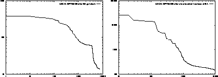
Figure: Two possible uses of Local-Optimize
. In the first example it
is used to refine the search after the genetic algorithm was stuck. In the
second example it is started after the genetic algorithm found a good region in
a few hundred iterations
The two examples shown in Figure are different runs of the
Local-Optimize
algorithm. The starting point for the first graph is the
best solution found by the genetic algorithm with problem-specific
modifications. The genetic algorithm discovered this solution in
13175 function evaluations and later got stuck. Local-Optimize
was started at that point and it was able to improve the error value about more than an order of magnitude. This example illustrates the difficulty with locating exact optima with the genetic algorithms. From the point the genetic algorithm got stuck, Local-Optimize was able to find a way further down in the error space. This demonstrates the importance of being able to do a fine grained search by shrinking the step sizes.
For the second graph, the genetic algorithm was run for a few hundred iterations. At that point it was stopped, and Local-Optimize
was started from the best point discovered so far. After about a thousand more function evaluations, the error was reduced to 370. This value is better than what the genetic algorithm got by itself in 13175 iterations.
The genetic algorithm is able to find good regions of the search space quickly by using problem-specific knowledge. However it is very inefficient in finding the optimum point in that region. The approach this suggests is to use problem-specific knowledge to locate the good regions in the space, and then to run Local-Optimize to find the exact location of the optima.