4. Bootstrapping Acquisition

**Figure 4.1:** Interdigitating learning and processing to bootstrap acquisition.
$\begin{figure} \centering \fbox{\psfig{file=figures/bootstrap.ps,height=2in}}\end{figure}$

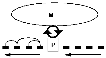
This chapter presents a bootstrapping mechanism for learning to identify linguistic relations. The key to the mechanism is to interdigitate learning and processing. That way the structures built by the processor can help the learner detect higher level regularities. Figure 4.1 depicts this feedback loop between the memory and the processor.

In the beginning of the training process, the processor cannot build any structure and the memory is presented with the raw input. As the memory detects low level correlations in the raw input, the processor uses this information to assign simple structure. The simple structure enables the memory to detect higher level correlations, which in turn enables the processor to assign more complex structure. Using this bootstrapping mechanism, the program starts reading raw text with no initial knowledge and reaches 60% precision and 50% recall in content word links after training.

I describe the implementation of the processor in the first section and the memory in the second section. This is followed by quantitative results of the learning process and a critical evaluation of its shortcomings. The final section discusses related work.

4.1 Processor

The goal of the processor is to find the dependency structure that assigns a given sentence a high probability. In Chapter 3, I showed that the probability of a sentence is determined by the mutual information captured in syntactic relations. Thus, the problem is to find the dependency structure with the highest total mutual information. The optimum solution can be found in time O(n⁵). I use an approximation algorithm that is O(n²). The main reason for this choice was the simplicity of the resulting processor as well as its speed. The simplicity is important because in the architecture of Figure 4.1, the input to the memory consists of the states and the actions of the processor, rather than the raw input signal. In order to make learning easy, the processor should be simple, i.e. it should have a small number of possible states and a small number of possible actions. Below, I present both the approximation algorithm and the optimum algorithm.

Approximation algorithm

There are two possible actions of the simple processor: given two words, they can be linked or not linked. The two words under consideration constitute the state of the processor visible to the memory. The order in which words come under the processor's attention is determined by a simple control system.

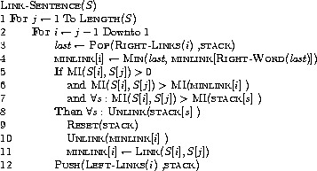
The control system reads the words from left to right. After reading each new word, the processor tries to link it to each of the previous words. When a link crossing or a cycle is detected, the weakest links in conflict is eliminated. Following is the pseudo-code for this n² algorithm:

$\begin{figure}\begin{tabbing} \par {\sc Link-Sentence}$(S)$\space \\ 1 {\bf For... ...{\sc Push}({\sc Left-Links}$(i)$ ,{\sc stack}) \\ \par\end{tabbing}\end{figure}$

The input S to the procedure LINK-SENTENCE is the sentence as an array of words. The links are created and deleted using LINK and UNLINK. The function MI gets the mutual information value for a link from the memory. The MINLINK array and the STACK are used to detect cycles and link crossings. The i th element of MINLINK contains the minimum valued link on the path from S[i] to S[j] if there exists one. As i moves leftward in the sentence, the right links of S[i] are popped and the left links of S[i] are pushed to the STACK. The last right link popped or the MINLINK on its right side becomes the new MINLINK[i]. A link crossing is detected when a new link is created with a nonempty stack. A cycle is detected when a new link is created when MINLINK[i] is nonempty.

Note that when a strong new link crosses multiple weak links, it is accepted and the weak links are deleted even if the new link is weaker than the sum of the old links. Although this action results in lower total mutual information, it was implemented because multiple weak links connected to the beginning of the sentence often prevented a strong meaningful link from being created. This way the directional bias of the approximation algorithm was partly compensated for.

To get a sense of how the link crossing and cycle constraints, combined with the knowledge of lexical attraction, lead to the identification of linguistic relations, a sequence of snapshots of the processor running on a simple sentence is presented below. Note that one or more steps may be skipped between two snapshots:

This algorithm is not guaranteed to find the most likely linkage. Also it can leave some words disconnected. Section 4.4 argues that the limiting factor for the performance of the program is the accuracy of the learning process due to representational limitations. Thus the marginal gain from an optimal algorithm would not be significant. The algorithm presented in this section performs reasonably well on the average and its speed and simplicity make it a good candidate for training.

Optimal algorithm

A Viterbi style algorithm [Viterbi, 1967] that finds the dependency structure with the highest mutual information can be designed based on the decomposition given in the proof of Theorem 2. The relevant figure is reproduced below for convenience:

$\begin{picture}(350,50) \put(0,0){$w_0$ } \put(40,0){$w_1$ } \put(60,0){$\ldots$... ...)[t]} \put(70,10){\oval(130,40)[t]} \put(150,10){\oval(290,60)[t]} \end{picture}$

Let $\sigma(h,a,b)$ be the dependency structure that gives the highest mutual information for the span w_a^b dominated by a word w_houtside this span. For convenience, I assume that the leftmost word dominates the whole sentence as in Theorem 2. Thus, the optimal algorithm must find $\sigma(0,1,n)$ . Let $\alpha(w_a^b \vert w_h)$ be the probability $\sigma(h,a,b)$ assigns to the span w_a^bdominated by w_h. For spans of length 1 and 0, $\alpha$ is given by:

$\begin{eqnarray*}\alpha(w_a^a \vert w_h) & = & P(w_a \vert w_h) \makebox[20pt]{} h \ne a \\ \alpha(w_a^b \vert w_h) & = & 1 \makebox[60pt]{} b < a \end{eqnarray*}$

Given the $\alpha$ values for spans of length up to l-1, the algorithm can compute it for spans of length l as follows:

$\begin{eqnarray*}\alpha(w_a^b \vert w_h) & = & \max_{i,j} P(w_i \vert w_h) \al... ..._a^{j-1} \vert w_h) \makebox[20pt]{} a \le j \le i \le b < h \\ \end{eqnarray*}$

Thus, the algorithm can compute the $\alpha$ values bottom up, starting with shorter spans and computing the longer spans using the previous $\alpha$ values. For each $\alpha$ value, the corresponding $\sigma$ structure can be recorded. At the end the structure $\sigma(0,1,n)$ gives the answer.

The recursive computation for $\alpha(w_a^b \vert w_h)$ takes O(n²)steps. For each length l from 1 to n, $\alpha$ must be computed for every span of length l and every possible head for each span, which means O(n³) $\alpha$ computations. Thus the total computation is O(n⁵).

4.2 Memory

The memory is a store of lexical attraction information. The lexical attraction of a word pair is computed based on the frequency with which the pair comes to the processor's attention. This information is then used by the processor when deciding whether to link two words. In this section I describe three different procedures for updating the memory. In the next section, I present the performance results of these three procedures.

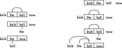
The memory may record pairs when the processor is in a certain state and ignore pairs that appear in different states. Different memory updating procedures can be created by choosing different states in which to record. Diagram (15) illustrates the first procedure. The memory records only pairs that are adjacent in the input. The three lines show three different time steps and the two windows show the words that the processor is trying to link.

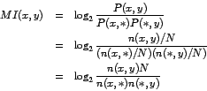
The basic data structures in the memory are words and word pairs with their counts. The same word may appear in the same window more than once as the processor tries to link it with different words. To keep a consistent count, each word keeps track of how many times it was seen in the left window and how many times it was seen in the right window, in addition to how many times it actually appeared in the text. Then the lexical attraction of two words can be estimated as:

$\begin{eqnarray*}MI(x,y) & = & \log_2 \frac{P(x,y)}{P(x,*) P(*,y)} \\ & = & \lo... ...,*)/N)(n(*,y)/N)}\\ & = & \log_2 \frac{n(x,y) N}{n(x,*) n(*,y)} \end{eqnarray*}$

where MI is mutual information, * is a wild-card matching every word, P(x,y) is the probability of seeing x on the left window and seeing y on the right window, n(x,y) is the count of (x,y), N is the total number of observations made in both windows.

A significant percentage of syntactic relations are between adjacent words. Using the first procedure, the program can discover the syntactic relations that are generally seen between adjacent words. For example, it can relate determiners and adjectives to nouns and learn collocations such as ``The New York Times''. Diagram (16) illustrates how the program learns to relate a determiner to its noun.

However, using this technique the program will never learn the relationship between kick and ball. A determiner almost always intervenes. There are other relations between words which are practically never seen next to one another. For example a prepositional phrase modifying a transitive verb is always hidden behind an object.

The second procedure for memory updating is to record all word pairs encountered, no matter how far apart in each sentence. Although this procedure is guaranteed to see every related word pair at some point, it also records a lot of unrelated pairs. The next section shows that even though this improves recall, the precision drops as expected.

Neither of the two procedures make use of the actual structure identified by the processor. In fact there is no feedback loop between the processor and the memory, thus no real interdigitation of learning and processing. The memory gathers its information looking at raw data and feeds it one way to the processor.

The third procedure is based on the feedback idea. The memory only records a subset of the pairs selected according to the structure identified by the processor. Before there is any structure, the memory behaves as in the first procedure, recording only adjacent pairs. If AXB is a sequence of three words, then the pairs A-X and X-B are recorded. When two words are linked, they form a group. In a sense, they act like a single word. If AX $\ldots$ YB is a sequence of words and X is linked to Y, the processor tries linking words in this group to both A and B. Because of the link crossing rule, words between X and Y cannot be linked^4.1. So, in addition to the adjacent pairs A-X and Y-B, the processor attempts to link A-Y and X-B. The memory records these pairs.

Diagram (17) shows how the third procedure leads to the discovery of the relation between kick and ball. In the left figure, the program uses the rule given in the previous paragraph and updates the pairs kick-ball and the-now. The kick-ball pair will be frequently reinforced and its high mutual information will be detected. The the-now pair will not be seen together much more than expected, so its mutual information will stay low. The right figure illustrates how the long distance link is formed once the correlation is identified. The next section shows that interdigitating learning and processing improves both precision and recall.

4.3 Results

This section presents results on the accuracy of the program in finding relations between content-words. I chose to base my evaluation on content-word links because they are essential in the extraction of meaning. Content words are words that convey meaning such as nouns, verbs, adjectives, and adverbs, as opposed to function words, which convey syntactic structure, like prepositions and conjunctions. The mistakes in content-word links are significantly more important than the mistakes in function-word links. The two sentences in (18) illustrate the difference. In the first sentence, a mistake would result in choosing the wrong subject for flying. In the second sentence, once the program has detected the relation between money and education, which way the word for links is less important.

Figure 4.2 shows the results of the three procedures described in the previous section. All three programs were trained using up to 100 million words of Associated Press material. After training they were presented with 200 sentences of out-of-sample test data and precision and recall were measured. The 200 out of sample sentences were hand parsed. There were a total of 3152 words, averaging 15.76 words per sentence, and 1287 content-word links in the test set. The choice of content-word links as an evaluation metric is also significant here. Most people agree on which content words are related in a sentence, whereas even professional linguists argue about how to link the function words.

**Figure 4.2:** Content-word link accuracy results
$\begin{figure} \centering \mbox{\psfig{file=figures/results.bigram.ps,width=2.9i... ... } \\ \mbox{\psfig{file=figures/results.feedback.ps,width=2.9in} } \end{figure}$

There are two sources of mistakes for the program. It can miss some links because there is an unknown word in the sentence. Or it can make mistakes because of the failure of the processor or the learning paradigm. In order to isolate the two, the test sentences were restricted to a vocabulary of 5,000 most frequent words, which account for about 90% of all the words seen in the corpus.

Accuracy is measured with precision and recall. Recall is defined as the percentage of content-word links present in the human parsed test set that were recovered by the program. Precision is defined as the percentage of content-word links given by the program which were also in the human parsed test set.

To help the reader judge the quality of these results, I will give some numbers for comparison. In the algorithm described above, the processor consults the memory for the lexical attraction of two words every time it is considering a new link. When the program is modified such that these numbers are supplied randomly, the precision is 8.9% and the recall is 5.4%, which gives a lower bound.

The program relies on the assumption that syntactically related words are also statistically correlated. Of the 1287 pairs of words linked by humans in the test set, 85.7% of them actually had positive lexical attraction, which gives an upper bound on recall.

4.4 A critical evaluation

In this section I present a qualitative analysis of the program's shortcomings and suggest future work. The mistakes of the program can be traced back to three main reasons:

Link types and second degree models

The relation between work and building in the two sentences are different. This is marked by using different prepositions. In general, language can use word order, function words, or morphology to represent different relations.

My program cannot represent this difference because it does not have different link types and its independence assumptions do not permit the representation of relations involving more than two words. In the examples above, the relation between two words is mediated by a third word, the preposition. The distribution of in the building, is different from just the building. A natural extension of my approach would be to relax the independence assumptions one step and to look at second-degree relationships, i.e. the modifiers of two words should influence their lexical attraction and should be used to mark the type of link between them.

Argument structure and using history

Another related source of mistakes for the program is to link strongly attracted words no matter how many other links they already have. Because there is no representation of different link types, the program cannot distinguish complements (mandatory arguments), from adjuncts (optional arguments). It can link four direct objects to a verb, or have a determiner modify three nouns simultaneously. After it learns to represent different link types, the solution would be to use the usage history of a word to learn its argument structure, and use this information to constrain its relations.

This solution could also help the opposite problem. The program cannot link the words it has never seen together before. Chomsky's sentence is the ultimate example: ``Colorless green ideas sleep furiously.'' The program would not be able to find any relations in this sentence no matter how much training it goes through (unless it comes across some linguistics textbooks). Although in real data no sentence is quite that bad, 15% of the relations are between words that do not have positive lexical attraction as pointed out in Section 4.3. Learning from the usage history of words and using this knowledge in less familiar situations is one solution to this problem.

Categorization and generalization

I stayed away from word categories in this work, partly because I think they have done more harm than good in the past. However, the existence of word categories and their regulatory role in syntactic constructions cannot be denied, although I believe we need a much finer system of type hierarchy than the current subcategorization frames and dictionary features allow.

Learning about each word individually has many advantages. However, no matter how much data is used, some words will be seen few times. One way to estimate the argument structure or the lexical attraction information for rare words is to identify their category from the few examples seen, and generalize the properties of this category to the rare word.

In addition to providing a solution to low sample problem, categorization of words is interesting in its own right. A lot of useful semantic information can be gathered by reading free text. For example, after reading ten years of Wall Street Journal, a program could discover that there is a category corresponding to our concept of politician, its members include the president, the prime-minister, the governor, their frequent actions include visiting, meeting, giving press releases etc.

There have been attempts to cluster words according to their usage, see for example [Pereira and Tishby, 1992,Brown et al., 1992,Lee, 1997]. However their success has been limited partly due to the lack of a good model to identify syntactic relations in free text. My approach is particularly suitable for this line of work.

4.5 Related work

Most work on unsupervised language acquisition to date has used a framework originally developed for finite state systems, i.e. (hidden) Markov models and used in speech recognition. The pillars of this approach are two algorithms for training and processing with probabilistic language models. The Viterbi algorithm selects the most probable analysis of a sentence given a model [Viterbi, 1967]. The Baum-Welch algorithm estimates the parameters of the model given a sequence of training data [Baum, 1972]. These algorithms are generalized to work with probabilistic context free grammars in addition to HMM's [Baker, 1979]. The Baum-Welch is sometimes called the forward-backward algorithm in the context of HMM's and the inside-outside algorithm in the context of PCFG's. For a detailed description of these algorithms, see [Rabiner and Juang, 1986,Lari and Young, 1990,Charniak, 1993].

The general approach is to define a space of context-free grammars and improve the rule probabilities by training on a part-of-speech tagged and sometimes bracketed corpus. Different search spaces, starting points, and training methods have been investigated by various researchers. Early work focused on optimizing the parameters for hand-built grammars [Jelinek, 1985,Fujisaki et al., 1989,Sharman et al., 1990]. Lari and Young used the inside-outside algorithm for grammar induction using an artificially generated language [Lari and Young, 1990]. Their algorithm is only practical for small category sets and does not scale up to a realistic grammar of natural language. Carroll and Charniak used an incremental approach where new rules are generated when existing rules fail to parse a sentence [Carroll and Charniak, 1992a,Carroll and Charniak, 1992b]. Their method was tested on small artificial languages and only worked when the grammar space was fairly restricted. Briscoe and Waegner started with a partial initial grammar and achieved good results training on a corpus of unbracketed text [Briscoe and Waegner, 1992]. Pereira and Schabes started with all possible Chomsky normal form rules with a restricted number of nonterminals and trained on the Air Travel Information System spoken language corpus [Pereira and Schabes, 1992]. They achieved good results training with the bracketed corpus but the program showed no improvement in accuracy when trained with raw text. Even though the entropy improved, the bracketing accuracy stayed around 37% for raw text. Figure 4.3 gives the accuracy and entropy results from this work.

**Figure 4.3:** No improvement in accuracy when trained with raw text.
$\begin{figure} \centering \mbox{\psfig{file=figures/pereira1.ps,width=2.9in}\psfig{file=figures/pereira2.ps,width=2.9in} } \end{figure}$

In general these approaches fail on unsupervised acquisition because of the large size of the search space, the complexity of the estimation algorithm and the problem of local maxima. Charniak provides a detailed review of this work [Charniak, 1993]. More recent work has focused on improving the efficiency of the training methods [Stolcke, 1994,Chen, 1996,de Marcken, 1996].

**Figure 4.4:** Phrase structure representation makes it difficult to get out of local maxima.
$\begin{figure} \centering \fbox{\psfig{file=figures/demarcken.ps,height=2in}}\end{figure}$

de Marcken [de Marcken, 1995] has an excellent critique on why the current approaches to unsupervised language learning fail. His main observation is that the phrase structure representation makes it difficult to get out of local maxima. His other observation is that early generalizations commit the learning programs to irrecoverable mistakes. Figure 4.4 illustrates the impact of the representation on the learning process. Two different structures for the string ABC are presented. A modifies B in one of them and B modifies A in the other. If the learner has chosen the wrong one, three nonterminals must have their most probable rules simultaneously switched to fix the mistake.

My work contrasts with these approaches in two important respects. First, most previous work uses part of speech information rather than words themselves. Recent work on high performance probabilistic parsers confirm that detailed lexical information is needed for high coverage accurate parsing [Magerman, 1995,Collins, 1996,Charniak, 1997]. Second, the standard formalism is focused on learning a probability distribution over the possible tree structures. My work simply assumes a uniform distribution over all admissible trees and concentrates on learning relationships between words instead.